ML Tutorial: Weka Part 3 – Predictions with Support Vector Machine

Getting started
Another very common machine learning algorithm is a Support Vector Machine or SVM. In the simplest terms it splits the data into groups using a separation line which is then used to predict which side a new data point is placed on.
In Part 1 of this series Weka performed feature selection. In Part 2 Weka’s IBk algorithm was tuned and used for predicting the volume of new product sales.
Here we use Weka’s Support Vector Machine.
SVM: Support Vector Machine
Instead of a neighborhood deciding similarity, the support vector machine algorithm seeks to find the widest possible margin that separates classes.
This is easiest to visualize when there are just two classes and they are linearly separable. A straight line is drawn separating the classes in such a way that it maximizes the distance between the nearest point of each class and the line itself. In other words a line that is the center of the largest margin between two classes.
In our case there are as many classes as there are existing products. So the SMOreg function in Weka will perform something called the one vs one reduction (OVO).
To understand OVO imagine we have only three products: A,B and C. OVO begins by first separation these three products into n(n-1)/2 combinations of binary classifications: (AB, BC, AC). Then when a new product is introduced it is compared to each of these binary classifications to see where it belongs.
Tuning the Algorithm
After choosing the SVMreg algorithm Weka can easily be used to tune its parameters for best results. In this case Weka provides ready access to the complexity parameter C, the kernel type, and whether or not the data is first normalized and or standardized.
Tuning kNN Complexity in Weka
C is known as the complexity parameter. It controls the sensitivity, or the degree of mistakes allowed, by the flexibility of the drawn line when separating classes. A small value of c, say 0, means that no violations of the margin are allowed, there must be a precise separation. In this case the algorithm is said to be too sensitive to the training data and overfitting occurs. A larger value for c means some miscalculations are allowed but the tuned model is more generalized as does a better job with new instances.
Choosing the kNN Kernel
It is often the case data is not linearly separable and some linear algebra is needed to transform the data into some Z space where separation can be done. Once done this same algebra is performed on each new instance before a calculation is made. There is an excellent visualization of a polynomial kernel where the original data is transformed in such a way that it can be clearly separated. The transformation does not permanently change the data. Instead it holds the transformation in memory long enough to perform the classification then releases it back to its original form. The two kernels we experiment with here are: polynomial and radial kernels.
Normalization/Standardization in Weka
Data often contains attributes that have wildly varying scales. One attribute might have values between 0 and 1 and another attribute might have values between 0 and 10,000. Both of the techniques we will use to train the SVM will create temporary relative values of the attributes.
Data normalization is the act of rescaling data into the range between 0 and 1. This means the largest possible value for any attribute is 1 and the smallest possible value is 0.
Standardization is the act of rescaling your data such that they have a mean value of zero and a standard deviation of 1. In both of these cases, like the kernel above, the data is not permanently altered, nor does the temporary change alter the relative relationships between the values.
Impact of Feature Selection in kNN
In this case we will tune the SVM algorithm on two different sets of data. We will run it on the original data with all attributes present and then on the set with the reduced number of features to see if there is a difference.
In Weka
- Select Explorer
- Click: Open File
- Choose existing_product_attributes_reduced_features.arff (from Part 1)
- Click: Open
- Click: Classify
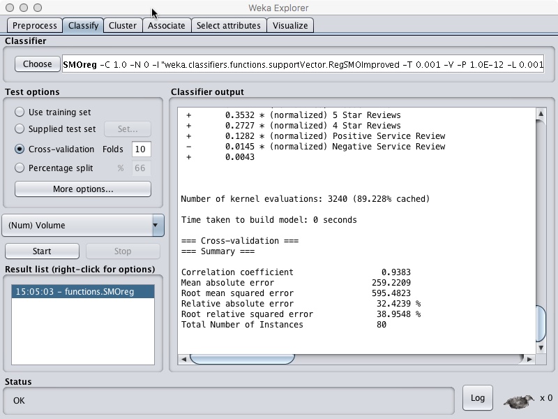
- Under Classifier: Choose functions>SMOreg
- Click: Close
- Confirm cross-validation Folds = 10
- Right-click on the text box to to the right of the choose button
- Under Kernel choose Polykernel
- Click Close
- Set c = 1
- Set Filter Type to Normalize training data
- Click OK
- Click Start
If we repeat this with the file that contains all the attributes for the existing products and continuously change the values of C, filter and kernel we can compile a list of results that look like this.
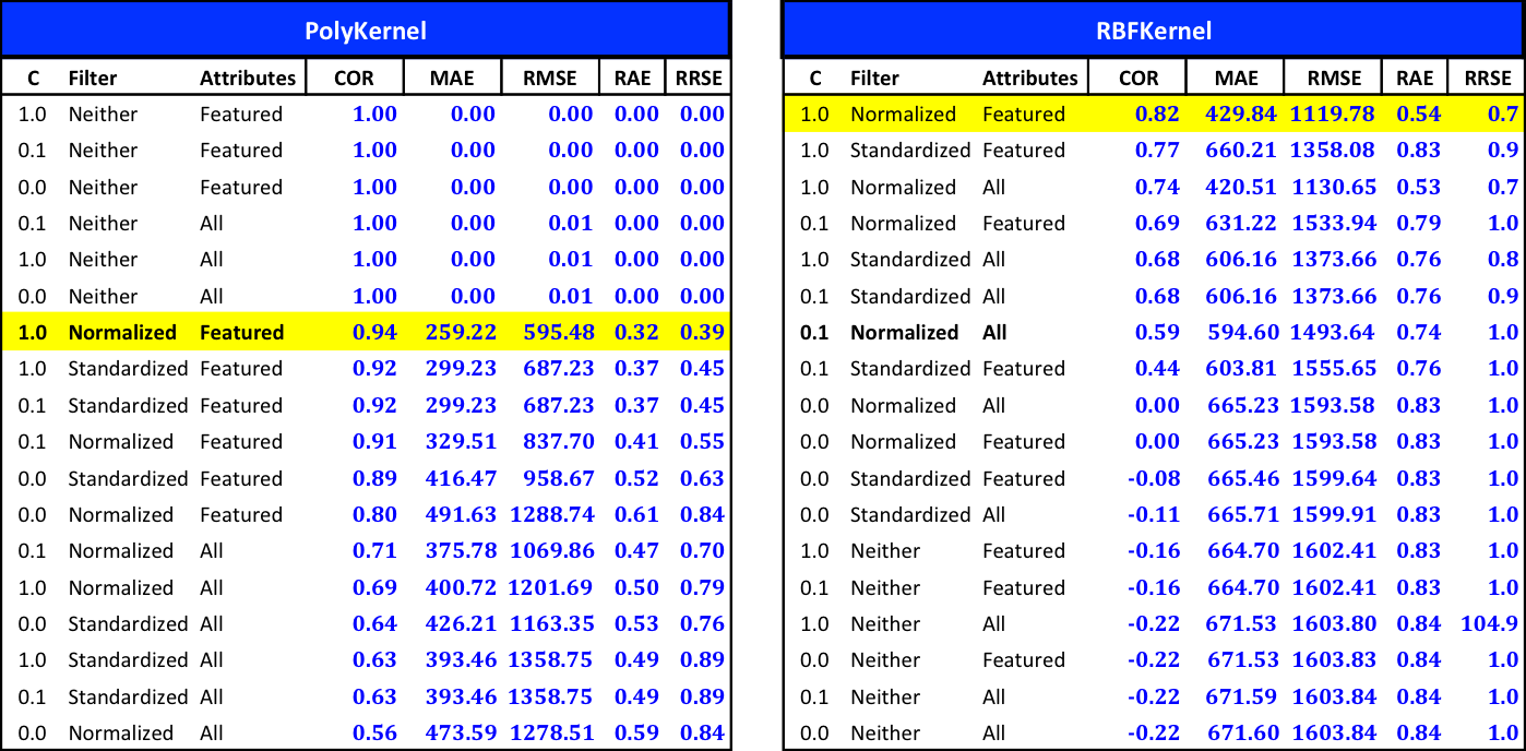
Notice the first 6 rows of the PolyKernel results. We see a correlation of 1 with zero errors. This is understood to mean that this configuration of the Algorithm has resulted in an overfitted model. This particular configuration is not considered in when judging the sorted results.
Support Vector Machine Prediction
We have tested a variety of tuning sets and found the two best configurations of SVM. We will now use these findings to preform the predictions.
First let’s confirm our settings for the SVMreg algorithm are those we want to use: Classifier=SVOreg; filter type = Normalize training data; c=1.
In Weka
- Under Classifier: Choose functions>SMOReg
- Click: Close
- Left-click the text box to the right of the choose button
- Change c=1
- Confirm filter type=Normalize training data
- Under kernel: Choose PolyKernel
- Click Close
- Click OK
- Click Start
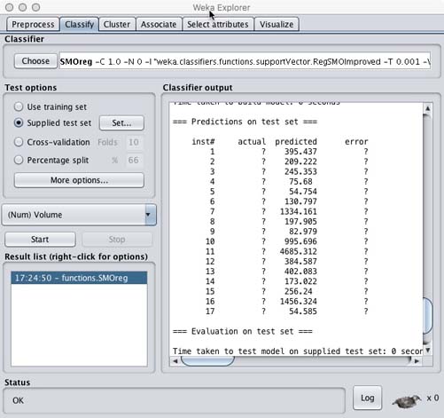
- Under Test Options: Choose Supplied Test Set
- Click Set
- Click Open file
- Choose new_product_attributes_reduced_features.arff (from Part 1)
- Click Close
- Click More options
- Under Output predictions click Choose
- Select Plain Text
- Click OK
- Click Start
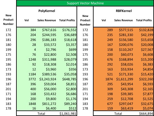
PolyKernel
To run the second best tuning set confirm settings as classifier=RBFKernel; filter type = Normalize training data; c=1.
We can then resolve the instance with the new product number in the spreadsheet, order the results by profits and present this to the business.
Summary
We began by testing a variety of parameters to tune each of 2 different kernels in the SVOreg algorithm in Weka. We captured values for the two best tuning parameter sets and ran those against our test set (new products). We got different values for all of the new products listed. However, if we ignore the actual values we find the products match in order of importance which is very similar to Weka Part 2.
Resources
Alexandre KOWALCZYK has a series of tutorials on SVM that are relatively self contained.
Abu-Mostafa gives a much more rigorous explanation of Support Vector machines in his online course. In particular starting with Lecture 14 Support Vector Machines and continuing through Lecture 15 and 16.
Machine Learning series beginning with Lecture 12.1.